How cubic interpolation works
In cubic interpolation, a 3rd order polynomial is used within an interpolation interval [P[n].X ... P[n+1].X] to calculate a value Y and its derivatives for a value X within the considered interval. A 3rd order polynomial is described by the following mathematical equation:
y = f(x) = a0 + a1 * x + a2 * x2 + a3 * x3
To determine the coefficients a0 ... a3, the following boundary conditions can be applied:
- Position at the left boundary:
P[n].Y = f(P[n].X) - Position at the right boundary:
P[n+1].Y = f(P[n+1].X) - Derivative at the left boundary:
y' = f'(P[n].X) - Derivative at the right boundary:
y' = f'(P[n+1].X)
The derivatives at the boundaries are estimated using the gradient of the straight line through the two neighboring points:
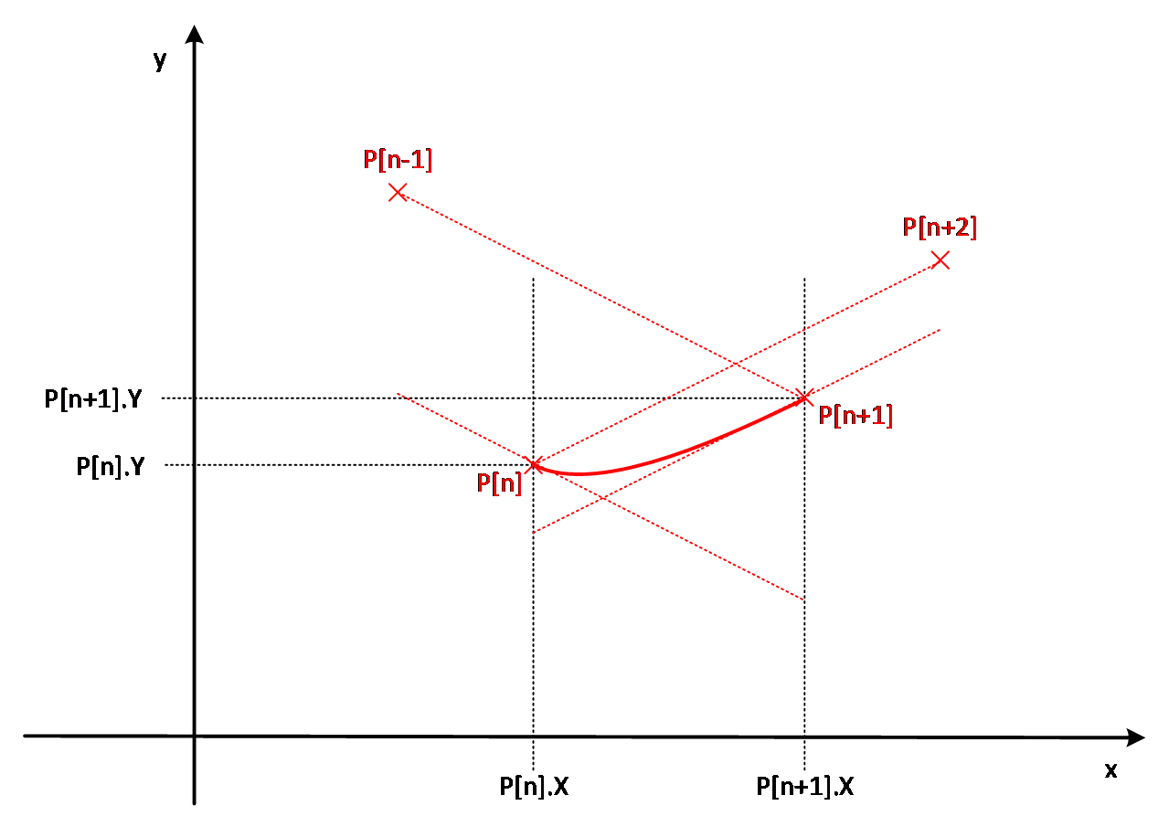
f'(P[n].X) = (P[n+1].Y - P[n-1].Y) / (P[n+1].X - P[n-1].X)
(gradient in P[n] = gradient of the straight line through P[n-1] and P[n+1])
f'(P[n+1].X) = (P[n+2].Y - P[n].Y) / (P[n+2].X - P[n-1].X)
(gradient in P[n+1] = gradient of the straight line through P[n] and P[n+2])
The following figure illustrates the procedure:
The procedure for estimating the derivative can easily be applied to any point within the point list. At the margin points, however, the problem arises that no preceding or subsequent point is defined. For this reason, other mechanisms that can be controlled via the eInterpolMode parameter are used at the margins to estimate the derivative.
